
[ WAA Home | ProjeX Home | Download ProjeX | Help using ProjeX | ProjeX FAQ | About WAA]
![]()
PERT Charts
In 1958, the Special Projects Office of the US Navy developed the Program Evaluation and Review Technique (PERT) to plan and control the Polaris missile program.
PERT is similar to CPA but has a probabilistic approach that allows three time estimates for the duration of each activity.
Our first step is to decide what our tasks are and which tasks depend on which.
Providing accurate estimates of task durations is not always easy without good historical data. For this reason the PERT approach uses three estimates for the duration of a task (activity).
PERT duration estimates:
Optimistic time (a): Time an activity will take if everything goes perfectly
Most likely time (m) : Most realistic time estimate to complete the activity
Pessimistic time (b) : Time an activity take if everything goes wrong
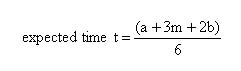
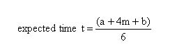
From these we calculate the expected time (t) for the task.
The time estimates are often (but not always, see below) assumed to follow the beta probability distribution:
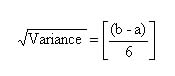
The project variance is the sum of the variances of each of the tasks on the critical path. The square root of this is the project standard deviation.
From the normal distribution equation:
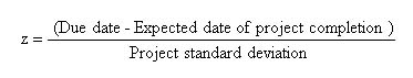
Looking this value up in the normal distribution tables gives the probability of the project being completed on our due date.
At the end of this process we have :
An expected completion date for the project
We know which tasks are critical to the project, ie. if they are delayed the delivery of the final product is delayed.
We know which tasks are not that critical, ie. they can be delayed to some extent (the float of the task) without affecting the overall delivery of the final product. Resources from these tasks could be diverted to the critical tasks if they start to fall behind.
We can get an estimate of how likely it is that the project will be finished by the deadline.
NOTE : It is not necessarily accepted that the normal distribution curve is suitable for predicting the spread of duration errors. Estimates are often too optimistic rather than too pessimistic so we would need to skew the distribution curve to correct for this. The formula below might be used: